Home / Monte Carlo / Latitude Plots / Creating Latitude Plots - Part V
Creating Latitude Plots - Part V
From Excel click...
QXL Monte Carlo Tab > Contribution Tools > Latitude Plots
This is the fifth article in a series that covers Latitude Plots. Links to the previous articles are below.
Part I - Understanding Latitude Plots
Part II - Understanding Latitude Plots
Part III - Interpreting Latitude Plots
Part IV - Multiple Inputs and Latitude Plots
Latitude Plots are a visual representation of the expected variation region (of the inputs) as compared to the latitude window (of the outputs). In the previous four articles, we covered the concepts behind the Latitude Plot. Now we are going to dive into creating Latitude Plots in Quantum XL and the options therein.
For this example, we will use the same model as in Part IV. The model is a simple stack of three parts with two outputs. The first output is stack height and the second output is the ratio of Part B to the total height of the stack. The model is shown below.
To create a Latitude Plot, select "Quantum XL" - "Latitude Plot" from the menu bar. Quantum XL will then validate that the model is in the correct form. Examples of models not in the correct form would be models with no inputs, no outputs, no equations, etc. If the model is valid and includes two or more inputs, you will be shown a window which allows you to select the plot range and identify which variables are to be included in the analysis.
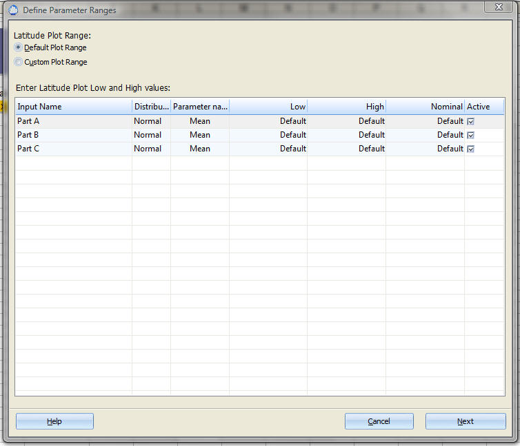
Latitude Plot Range
Default Plot Range - Quantum XL will select the scaling for the Latitude Plot to ensure that the entire expected variation region (red box) will be displayed with ample room around the box to view additional points. Note that when this option is selected, the columns "Low", "High", and "Default" will not be editable and will "Default".
Custom Plot Range - In the event that you would like to widen or reduce the plot range, you can use this option. When you click on this option, you will be able to edit the "Low" and "High" values for each input.
Options by Input
Each input has four columns that can be edited to control the way the chart is created. Note that the Input Name, Distribution, and Parameter columns are read-only.
Low and High - The Latitude Plot's minimum and maximum value for this variable. To change this value, "Custom Plot Range" must be selected.
Nominal - When the expected variation region (red box) is computed, the equations for the output depend on a value for all of the inputs. For this model, when the red box is calculated for Part A vs. Part B, the other variable (Part C) must have some value. This value is the nominal value and can be changed if you select "Custom Plot Range". If left as the default, the location parameter is used as the nominal value. For example, the location parameter for the Normal distribution is the mean. The nominal values are displayed in the Latitude Plot on the left side of the chart grid.
Note the words "Nominal = 18" displayed in the left border of the Latitude Plot below. Each input's Nominal value is displayed on the resulting Latitude Plot.
Active - Remove the check mark in this column if you want to exclude this input from the Latitude Plots to be created. Note that you can remove this check in either Default Plot Range or Custom Plot Range mode. The number of Latitude Plots will grow very quickly. The table below shows the number of Latitude Plots for various numbers of inputs.
| # Inputs | # of Latitude Plots | # Inputs | # of Latitude Plots | |
|---|---|---|---|---|
| 2 | 1 | 21 | 210 | |
| 3 | 3 | 22 | 231 | |
| 4 | 6 | 23 | 253 | |
| 5 | 10 | 24 | 276 | |
| 6 | 15 | 25 | 300 | |
| 7 | 21 | 26 | 325 | |
| 8 | 28 | 27 | 351 | |
| 9 | 36 | 28 | 378 | |
| 10 | 45 | 29 | 406 | |
| 11 | 55 | 30 | 435 | |
| 12 | 66 | 31 | 465 | |
| 13 | 78 | 32 | 496 | |
| 14 | 91 | 33 | 528 | |
| 15 | 105 | 34 | 561 | |
| 16 | 120 | 35 | 595 | |
| 17 | 136 | 36 | 620 | |
| 18 | 153 | 37 | 666 | |
| 19 | 171 | 38 | 703 | |
| 20 | 190 | 39 | 741 |
Latitude Plot Options
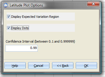
Display Expected Variation Region - Enables or disables the display of the Expected Variation Region (red box).
| Default Latitude Plot | Latitude Plot without Expected Variation Region |
|---|---|
 |
 |
Display Dots - Enables or disables the display of the red and blue dots. If you have many inputs, disabling the dots will make the Latitude Plots easier to read.
| Default Latitude Plot | Latitude Plot without Display Dots |
|---|---|
|
 |
Confidence Interval - Controls the size of the Expected Variation Region. The default value is .99 or 99% of the expected variation in the inputs. Valid values are from .1 to .999999. As you increase the confidence interval, the size of the expected variation region will increase.
| Distribution | Confidence Interval | Size of Expected Variation Region |
|---|---|---|
| Normal | .99 | Mean +/- 2.58*Standard Deviation |
| Normal | .999 | Mean +/- 3.29*Standard Deviation |
| Normal | .9999 | Mean +/- 3.89*Standard Deviation |
| Normal | .99999 | Mean +/- 4.42*Standard Deviation |
| Normal | .9999966 | Mean +/- 4.645*Standard Deviation (3.4 defects per million) |
| Normal | .999999 | Mean +/- 4.89*Standard Deviation |
To illustrate this, I have created the Latitude Plots for the model with both the .99 and .999999 confidence intervals. The Latitude Plots for Part A vs. Part B are displayed below.
| .99 Confidence Interval | .999999 Confidence Interval |
|---|---|
|
 |
Non-normal distributions are calculated using the appropriate probability distribution. For example, if you define an input to be Uniformly distributed from -1 to 1 or U(-1,1), then a .99 confidence interval would plot from -.99 to +.99.
Distributions with an offset parameter (e.g., Exponential, Gamma, Weibull, etc.) are calculated using a single sided confidence interval. The left side of the confidence interval will correspond to the offset parameter.