Home / Monte Carlo / Latitude Plots / Understanding Latitude Plots - Part II
Understanding Latitude Plots - Part II
From Excel click...
QXL Monte Carlo Tab > Contribution Tools > Latitude Plots
This is the second article in a series that covers Latitude Plots. A link to the previous article is below.
Part I - Understanding Latitude Plots
In the first article, Understanding Latitude Plots, we introduced Latitude Plots and discussed the basics. If you have not read the introductory article, I highly recommend that you click here.
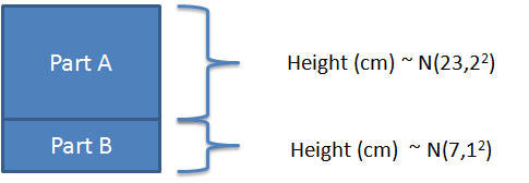
In this article, we will build on our existing model. Remember that we are working with a stack of two parts, each of which has the height shown in the graphic below.
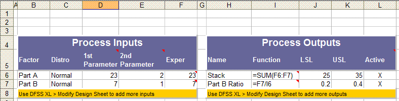
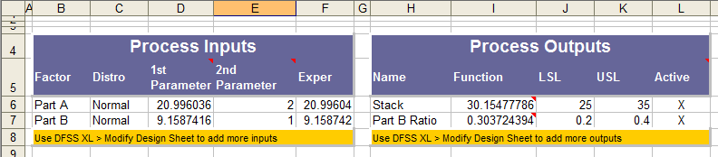
In Part I, we had only one output. The total stack height was required to be between 25cm and 35cm. Thus the Lower Specification Limit (LSL) and Upper Specification Limit (USL) are 25 and 35 respectively. In Part II, we want to include the requirement that the ratio of Part B to the total stack height be between 20% and 40%. To do this, we add another output with the equation F7/I6. The cell F7 contains the height of Part B and the cell I6 contains the height of the stack. Alternatively, we could have entered the equation =F7/Sum(F6:F7) with the same results.
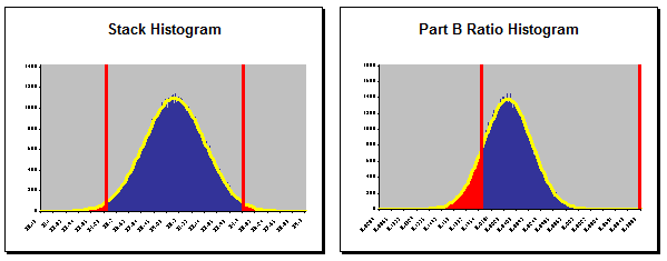
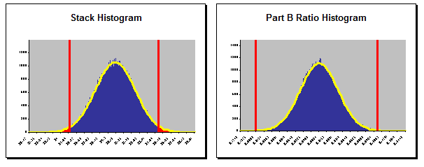
The Monte Carlo simulation results in the histogram below. The histogram for Part B Ratio shows significant defects below the LSL.
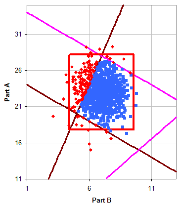
The Latitude Plot for this model is below. The purpose of a Latitude Plot is to show the expected variation region compared to the latitude window. In the first article, I explained that the red box is the expected variation region. A few observations about this Latitude Plot.
-
There is still only one Latitude Plot. When we have two outputs we get two histograms; however, Latitude Plots are created in pairs of inputs. Since we still have two inputs (Part A and Part B) we only have one Latitude Plot with both outputs depicted on the plot. If we had added another 10 outputs while maintaining 2 inputs, we would still only have one Latitude Plot.
-
The number of Latitude Plots created by Quantum XL is completely a function of the number of inputs. However, with additional outputs the number of specification limit lines on the Latitude Plot will increase.
-
Our expected variation region in Part II is identical to the region in Part I. This is because the variation in Part A and Part B is the same as in the previous article.
-
We have two additional lines that describe the latitude window. These lines represent the LSL and USL for the "Part B Ratio".
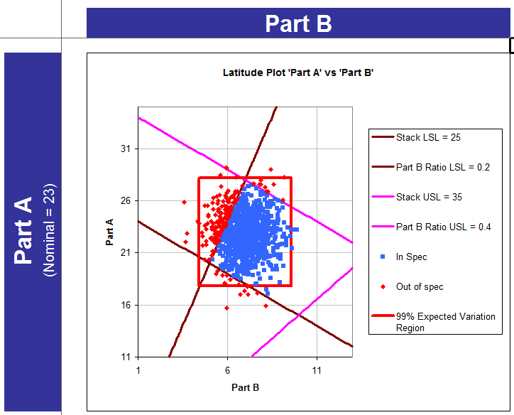
In the Latitude Plot found below, arrows have been added to show that the area combinations of Part A and Part B cause the output Part B Ratio, or "Ratio" for short, to be out of spec. The area between the lines that contains the blue dots represents the latitude window.
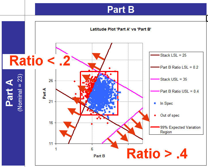
It is clear from looking at the plot that if we were to shift the square down and to the right we would have fewer defects. Quantum XL has an optimizer that can perform this function for us. I optimized the outputs by selecting "Quantum XL" - "Optimize (Param Design)". The optimizer has chosen a new mean (average) for both Part A and Part B. The new nominal value for Part A is 20.99 and for Part B is 9.16.
Below are the histograms before optimization and after.
Before Optimization - Part A~N(23,2²), Part B~N(7,1²)
After Optimization - Part A~N(20.99,2²), Part B~N(9.16,1²)
The Latitude Plot after optimization is shown below. This might not look very familiar, as the scale for Parts A and B has changed.
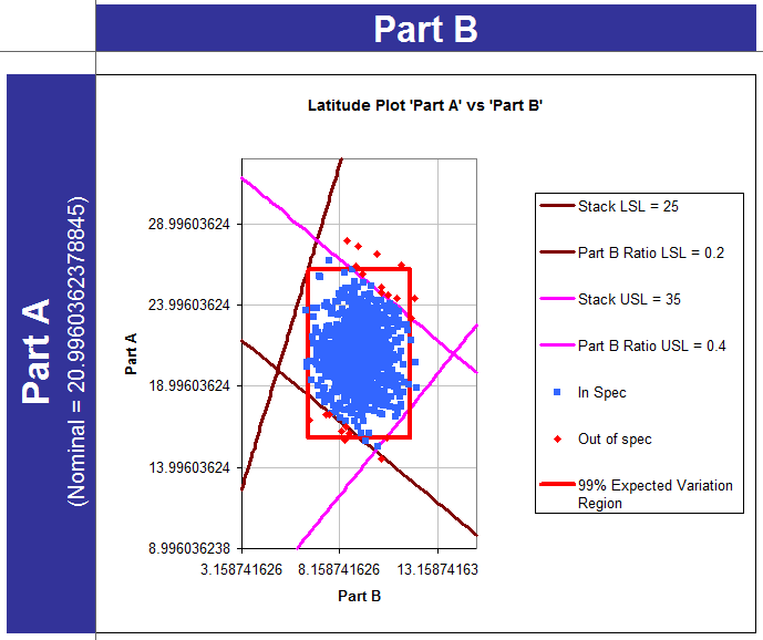
However, Quantum XL will allow you to choose a custom scale. A comparison of the Latitude Plots before and after optimization (with the same scale) is shown below.
| Before Optimization Part A~N(23,2²), Part B~N(7,1²) |
After Optimization Part A~N(20.99,2²), Part B~N(9.16,1²) |
|---|---|
 |
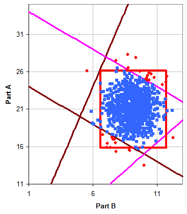 |
Using the Latitude Plots, it is easy to see how the optimizer reduced the defects by changing the mean. The expected variation window fits more completely in the latitude window resulting in fewer defects. In the next article, we will go over the interpretation of Latitude Plots.