Home / DOE / Analyze / Regression Results for Ordinary Least Squares

Regression Results for Ordinary Least Squares

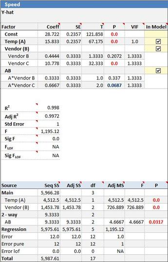
When you select Run Regression from QXL DOE Tab --> Analyze Design, Quantum XL will calculate the ordinary least squares regression and write the results to a new workbook. Below is an example of the regression results from a mixed level full factorial. Factor A (Temperature) is at two levels while Factor B (Vendor) is qualitative at three levels.

Coefficient

The coefficient for the term is the units of the model (usually coded). The default for all models, including historical data, is for Quantum XL to autocode the data between -1 and +1. As a result, the coefficients are for coded units. If you would like the regression results in uncoded coefficients, select QXL DOE Tab --> Analyze Design --> Uncoded Coefficients.

SE (Standard Error)

The standard error of the regression coefficient is a measure of the uncertainty of the coefficient. Smaller values indicate better estimates while larger values indicate the likelihood of more error. The standard error is mainly used in the calculation of the T Statistic.

T

The T value (T Statistic) is calculated as the absolute value of the coefficient divided by the standard error. In this manner, it is a Signal (coefficient) to Noise (SE) ratio with larger values indicating more signal than noise. The T Value is used in the calculation of the P-Value.

Larger values for T indicate that the coefficient is different from zero.

P

The P Value (P 2-Tail) is calculated by comparing the T Value to the t Distribution with the appropriate degrees of freedom. Smaller values of P indicate that the term is significant.

Quantum XL color codes the P-Values according to the following table.

• Less than .05 --> Red
• Between .05 and .1 --> Blue
• Greater than .1 --> Black

(1-p)*100% is the percent confidence the term is significant. Most researchers use p<.05 as the threshold for significance.

VIF (Variance Inflation Factor)

VIF is a measure of multicollinearity in a model.

Multicollinearity occurs when inputs are correlated with each other. Most DOEs will have VIFs=1 which indicate that the inputs are orthogonal (independent).

However, when working with regression models which originate from non-DOE sources, the VIFs are likely to be larger than 1.

As the VIFs increase from 1, the degree of multicollinearity increases. There is a great deal of debate over how much multicollinearity is too much. Some experts suggest that values over 2 are excessive while others draw the line at 10.

In cases of extreme multicollinearity, the coefficients can have gross errors to include the wrong sign. Subsequently, the p-values for these terms are also error laden. Insignificant terms can show as significant while significant terms appear insignificant. High VIFs should be avoided by removing correlated inputs before running the regression.

In Model

To remove a term from the model, remove the check mark and re-run the regression by selecting QXL DOE Tab --> Analyze Design --> Run Regression.

R²

R² reflects the strength of the model or the percent of the variation that can be explained by the model. R² will fall between 0 and 1. R² = 0 indicates a model where the inputs and outputs are not correlated (none of the variation in the input can be explained by the model). R² = 1 indicates a perfect model where 100% of the variation in the outputs can be explained by the model. Larger values are typically preferred, but R² should not be confused with the P value.

It is possible for the R² to be very low yet still have significant terms.

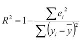
Where eᵢ is the ith residual, yᵢ is the ith output observation, and ȳ is the average y.

Adj R² (Adjusted R²)

Adjusted R² is an adjustment for R² to account for the number of output observations and the number of terms in the model.

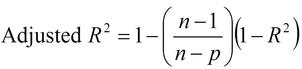
Where n = number of output observations and p = number of terms in the model. While R² always falls between 0 and 1, Adjusted R² can be a negative number.

For most Designed Experiments, Adjusted R² and R² will be very close. If there is a large difference between the two, it is an indication that your model has too few degrees of freedom (n is close to p).

F (F Statistic)

The F Statistic (F Value) is a measure of the predictive abilities of the entire model. F is essentially a signal to noise ratio. Larger values of F indicate more signal than noise. A large F value indicates a model that should predict well.

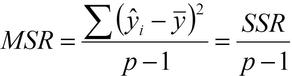
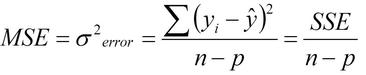
The equation for F is…

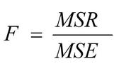
Where MSR = Mean Squared Regression and MSE = Mean Squared Error.

Sig F (Significance F)

Sig F provides a probability that the F value is larger than 1. An F value equal to 1 indicates that signal = noise and the model will not predict well. As F increases, Sig F will decrease, indicating better predictive capabilities. Many experimenters consider Sig F < .05 to indicate a significant model adequate for prediction.

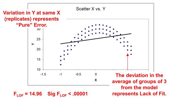
FLOF (F Lack of Fit)

F_LOF is a measure of Lack of Fit. A good example of a model with lack of fit is below. The data (blue dots) has a quadratic shape but the model is linear. The larger F_LOF indicates more lack of fit although you must be careful in interpreting as the degrees of freedom in the model must be used when deciding if your model has lack of fit. Use Sig F_LOF as a metric as it includes both F_LOF and the degrees of freedom.

Sig FLOF (Significance FLOF)

Sig F_LOF provides a probability that your model suffers from lack of fit. The calculation of Sig F_LOF includes both the F_LOF and the degrees of freedom in your model. If Sig F_LOF < .05, you can be greater than 95% confident that the model has lack of fit.

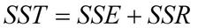
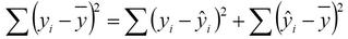
Sums of Squares

Quantum XL will calculate both the Sequential Sums of Squares (Type I) and Adjusted Sums of Squares (Type III).

Sequential Sums of Squares (Type I)

Sequential SS are calculated by removing the terms one by one from the model and noting the change in the residual sums of squares. For example, if a model includes the terms Const, A, B, and AB, then the Sequential Sums of Squares for the term AB is equal to the change in the residual sum of the full model and the model without the AB term.

The Sequential SS for the term B will be the difference between the model with Const, A, and B and the model with Const and A (i.e., B was removed).

Most experimenters prefer the Adjusted Sums of Squares (Type III) over the Sequential SS.

Adjusted Sums of Squares (Type III)

Adjusted SS reflects the reduction in residual SS for a full model and the model without the ith coefficient. Unlike the sequential SS, the Adjusted SS always compares the reduction with the model with all terms.

For example, if the full model includes the terms Const, A, B, and AB, then the Adjusted SS for the term A will be the difference in residual sums of squares for the full model and the model with A removed (Const, B, and AB remaining). The Adj SS for the B term is the difference in residuals from the full model and the term B removed (Const, A, and AB remaining).

Note

• If a design is orthogonal, the Seq SS will equal the Adj SS.
• Sequential SS are additive. The SS Regression is the sum of the Sequential SS.