Home / DOE / Analyze / Regression Results for Binary Logistic Regression
Regression Results for Binary Logistic Regression
When you select Run Regression from the QXL DOE Tab --> Analyze Design menu item, Quantum XL will calculate the binary logistic regression for all binary outputs and write the results to a new workbook.
Coefficient
The coefficient for the term is the units of the model (usually coded). The default for all models, including historical data, is for Quantum XL to autocode the data between -1 and +1. As a result, the coefficients are for coded units. If you would like the regression results in uncoded coefficients, select QXL DOE Tab --> Analyze Design --> Uncoded Coefficients.
To predict using the regression coefficients for binary logistic regression you must use the logit function.
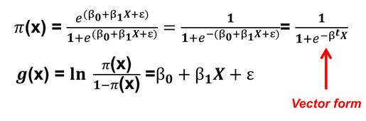
Where π(x) is the predicted probability and β is a vector of regression coefficients.
β₀ is the constant and β₁….βₙ are the input coefficients.
SE (Standard Error)
The standard error of the regression coefficient is a measure of the uncertainty of the coefficient. Smaller values indicate better estimates while larger values indicate the likelihood of more error. The standard error is mainly used in the calculation of the T Statistic.
Z (Z Statistic)
The Z value (Z Statistic) is calculated as the absolute value of the coefficient divided by the standard error. In this manner, it is a Signal (coefficient) to Noise (SE) ratio with larger values indicating more signal than noise. The Z Value is used in the calculation of the P-Value.
Larger values for Z indicate that the coefficient is different from zero.
P
The P Value (P 2-Tail) is calculated by comparing the T Value to the Z Distribution with the appropriate degrees of freedom. Smaller values of P indicate that the term is significant.
Quantum XL color codes the P-Values according to the following table.
- Less than .05 --> Red
- Between .05 and .1 --> Blue
- Greater than .1 --> Black
(1-p)*100% is the percent confidence the term is significant. Most researchers use p<.05 as the threshold for significance.
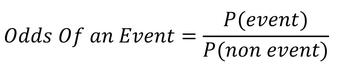
Odds Ratio
The odds of an event occurring is the probability that the event occurs divided by the probability that the event does not occur.
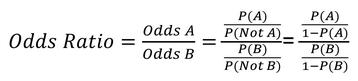
The odds ratio is used to compare the odds of two groups. For example, if Group A is treated differently than Group B the Odds Ratio for A vs. B would be…
Example: A video console company surveyed a sample and found the following.
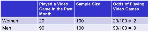
The Odds ratio between Men and Women for playing video games would therefore be.
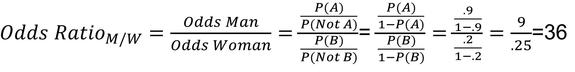
Odds ratio is historically used to understand the likelihood of two groups compared to each other. The literal interpretation of the Odds Ratio is that the odds of a man playing video games are 36 times greater than a woman. Care should be exercised when interpreting these results. In this example, men are .9/.2 = 4.5 times more likely to play video games but have 36 times the odds. Many experimenters think in terms of probability (not odds). If you want to compare probabilities, consider using the prediction area at the top of the regression table.
An Odds Ratio = 1 indicates that the two groups have equal probability. As the Odds Ratio moves away from one, either larger or smaller, the odds of one group is greater than the other.
95% CI Lower
The 95th percentile lower confidence interval for Odds Ratio.
95% CI Upper
The 95th percentile upper confidence interval for Odds Ratio.
In Model
To remove a term from the model, remove the check mark and re-run the regression by selecting QXL DOE Tab --> Analyze Design --> Run Regression.
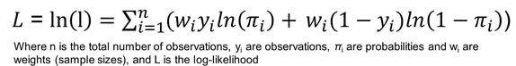
LogLikelihood
The natural log of the likelihood function or Ln(likelihood). Parameter estimation for logistic regression is calculated using Newton's algorithm which maximizes the ln(likelihood). The final value of the optimized function is reported as LogLikelihood.
RSquaredU
RSquaredU (McFadden's pseudo R²) is similar to the R² value in ordinary least squares. Larger values indicate a stronger model.
AIC (Akaike Information Criteria)
When comparing models, the lower AIC is generally preferred.
Note that Quantum XL calculates the AIC, not the corrected AIC (AICc).
AIC = 2k = 2ln(L) where k is the number of terms in the model and L is the maximized value of the likelihood function. The AIC penalizes the number of parameters less than the Bayesian Information Criteria.
BIC (Bayesian Information Criteria, Schwarz Criterion, SBC, or SBIC)
When comparing models, the lower BIC is generally preferred.
BIC =2Ln(L) + kLn(n) where L is the maximized value of the likelihood function, k is the number of terms in the model, and n is the number of data points in the design matrix x.
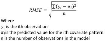
RMSE (Root Mean Square Error)
The root mean square error is measure of the deviation from observed and predicted.
G Stat
G is a test that all the slopes are equal. G is calculated as -2*(Ln(Lconst) - Ln(Lfullmodel)) where:
- Ln(Lconst) is the log-likelihood of the model with only a constant term
- Ln(Lfullmodel) is the log-likelihood of the full model
Larger G values indicate models with more slope. Use G P-value to determine significance.
G df
The degrees of freedom in the G statistic.
G P-Value
If the G-Pvalue < .05, you are at least 95% confident that the slopes are not all equal to zero (the model is significant for prediction).
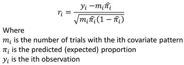
Pearson Goodness of Fit Test
Measure of how well the model fits the data, higher chi-sq values with p < 0.05 indicates a significant lack of fit. The Pearson statistic is calculated from the Pearson residuals (rᵢ). The Chi-Sq value is calculated as the sum of the rᵢ².
Deviance Goodness of Fit Test
Measure of how well the model fits the data; p < .05 indicates a significant lack of fit. The deviance statistic shouldn’t be used if the number of unique covariates is close to the number of observations. With more replications per covariate pattern, the deviance becomes more useful.
Measures of Association
Consider a pair of observations (x1,y1) and (x2,y2) and their predicted probabilities from the logistic model π1, π2. In this example, x1 and x2 are different rows in the input matrix X, y1 and y2 are the observed rate of occurrence, and π1, π2are the predicted probabilities for x1 and x2.
Concordant pairs
A pair, x1 and x2, are concordant if…
y1<y2 and π1< π2
OR
y1>y2 and π1> π2
or, equivalently…
sign(y1-y2) = sign(π1 - π2)
Discordant pairs
A pair, x1 and x2, are discordant if…
y1
OR
y1>y2 and π1< π2
or, equivalently…
sign(y1-y2) = -sign(π1 - π2)
Ties
A pair, x1 and x2, are a tie if y1 = y2.
Number/Percent of Concordant Pairs
For every covariate pattern in the model (rows in the X matrix) Quantum XL will determine if the pair is concordant, discordant, or a tie. The number of concordant pairs is a count of these pairs which were concordant. The more concordant pairs, the stronger the model.
Number/Percent of Discordant Pairs
For every covariate pattern in the model (rows in the X matrix) Quantum XL will determine if the pair is concordant, discordant, or a tie. The number of discordant pairs is a count of these pairs which were discordant.
Number/Percent of Ties
For every covariate pattern in the model (rows in the X matrix) Quantum XL will determine if the pair is concordant, discordant, or a tie. The number of ties is a count of these pairs which were ties.
Somers' D
A summary statistic calculated from the concordant and discordant pairs. Unlike Goodman-Kruskal Gamma, ties are not considered. Ranges from -1 (All Pairs Disagree) to +1 (All Pairs Agree). Higher values indicate stronger models.
Goodman-Kruskal Gamma
A summary statistic calculated from the concordant, discordant, and tied pairs. Unlike Somers' D, ties are considered. Ranges from -1 (All Pairs Disagree) to +1 (All Pairs Agree). Higher values indicate stronger models.
Kendall's Tau
A summary statistic calculated from the concordant and discordant pairs. Differs from Somers’ D in that it takes into account the difference between the numbers of possible paired observations. Kendall’s Tau is usually smaller than Somers’ D. Ranges from -1 (All Pairs Disagree) to +1 (All Pairs Agree). Higher values indicate stronger models.